Get Started

The following documentation walks through an example of using the ggplot2 R package and RStudio for basic data visualization. If you are new to R and want to learn more about using R for Data Science, also see the R for Data Science textbook which is available in print or as a freely available website

ggplot2 is part of the tidyverse ecosystem of packages.

The tidyverse is an opinionated collection of R packages designed for data science. All packages share an underlying design philosophy, grammar, and data structures.

Hello RStudio

RStudio is an integrated development environment (IDE) designed to help you be more productive in your daily data science work.

After you have installed R and RStudio, you are ready to begin this section!

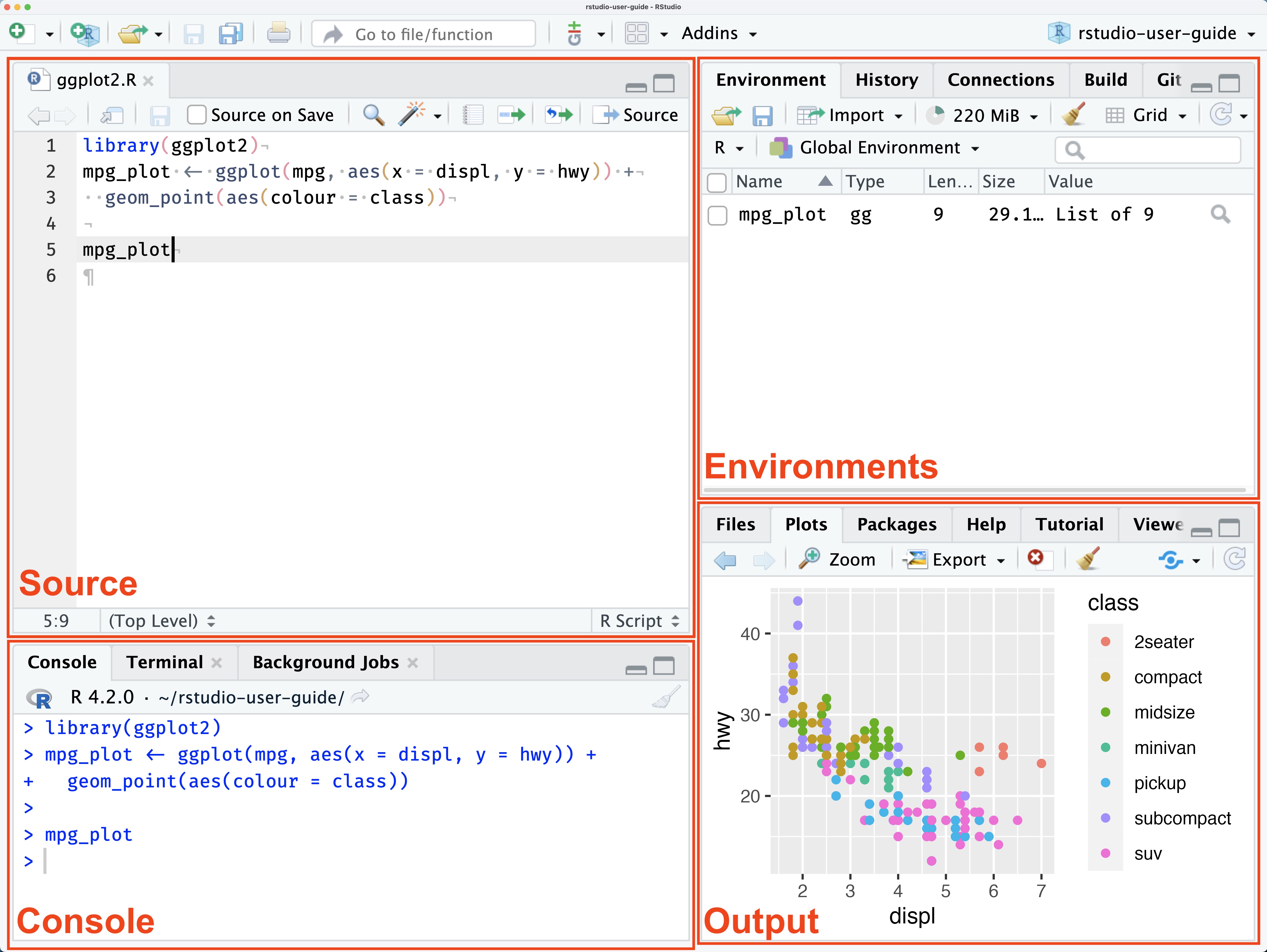
When you start RStudio, you’ll see four key regions or “panes” in the interface: the Source pane, the Console pane, the Environment pane and the Output Pane.

RStudio Panes

The Source pane is where you can edit and save R or Python scripts or author computational documents like Quarto and R Markdown.
The Console pane is used to write short interactive R commands.
The Environment pane displays temporary R objects as created during that R session.
The Output pane displays the plots, tables, or HTML outputs of executed code along with files saved to disk.

A screenshot of the RStudio UI. There are 4 primary panes, the source, console, environment, and output panes.

Blank slate

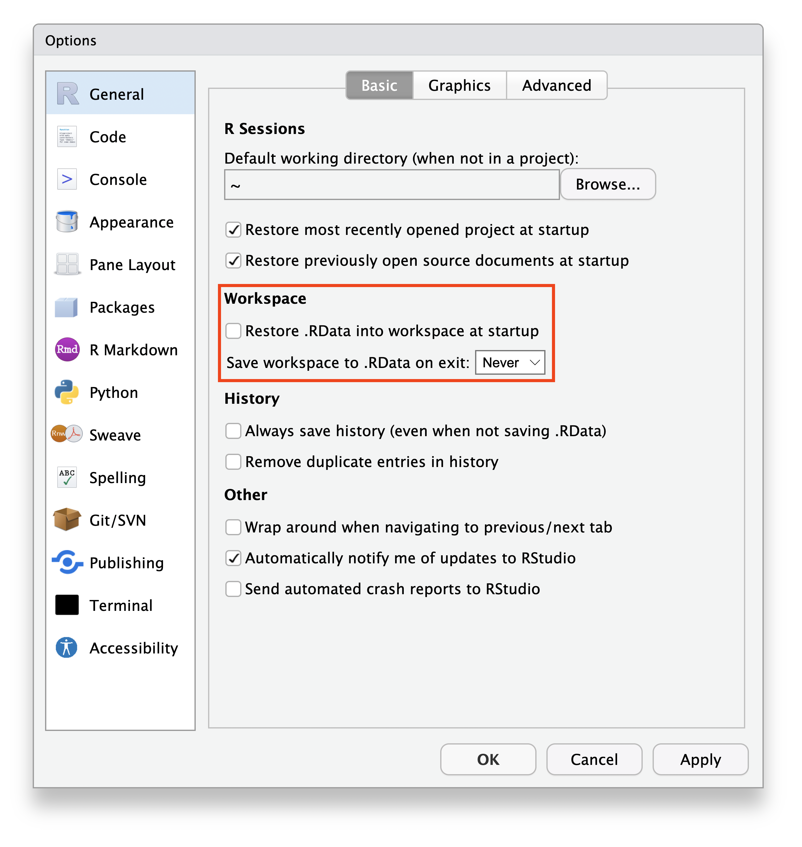
When you quit R, do not save the workspace to an .Rdata file. When you launch, do not reload the workspace from an .Rdata file. Long-term reproducibility is enhanced when you turn this feature off and clear R’s memory at every restart. Starting with a blank slate provides timely feedback that encourages the development of scripts that are complete and self-contained.

In RStudio, set this via Tools > Global Options, making sure to clear “Restore .RData into Workspace at Startup” and choosing Never on the “Save workspace to .RData on exit”.

Hello RStudio Projects

RStudio projects make it straightforward to divide your work into multiple contexts, each with their own working directory, workspace, history, and source documents.

To create a new project in the RStudio, use the File > New Project command.

In the New Project wizard that pops up, select New Directory, then New Project. Name the project “hello-ggplot2” and then click the Create Project button.

This will launch you into a new RStudio Project inside a new folder called “hello-ggplot2”.

RStudio projects give you a solid workflow that will serve you well in the future:

Create an RStudio project for each data analysis project.
Keep data files there; we’ll talk about loading them into R in Local Data.
Keep scripts there; edit them, run them in bits or as a whole.
Save your outputs (plots and cleaned data) there.

Everything you need is in one place, and cleanly separated from all the other projects that you are working on.

Hello `ggplot2`

The following section is adapted from the “Data Visualization” chapter of R for Data Science.

R has several systems for making graphs, but ggplot2 is one of the most elegant and most versatile.

Let’s get started creating a basic graph with R via ggplot2.

Install the ggplot2 R package by executing the below code via the R console

install.packages("ggplot2")

You only need to install a package once, but you need to load it with library() every time you start a new session.

In RStudio, create a new .R file and label it ggplot2.R via File Menu > New File > R Script

The ggplot2.R file you have just created will open in the Source Pane, which by default is in the top left.

Since you have already installed ggplot2, you can write the following code into the first line of your ggplot2.R script to load the ggplot2 package for that session.

library(ggplot2)

The library() function will load a specific R package (ggplot2) so you can use the R functions within it. In the case of ggplot2, it contains many functions for creating useful and elegant graphs in R.

To execute that code in the R console, you can move your cursor to the specific line of code and either use the Run command in RStudio or the Ctrl + Enter (Cmd + Enter on Mac) shortcut.

First Steps

Let’s use our first graph to answer a question:

Do cars with big engines use more fuel than cars with small engines?

We will be looking at the mpg data frame built into ggplot2. A data frame is a rectangular collection of variables (in the columns) and observations (in the rows). mpg contains observations collected by the US Environmental Protection Agency on 38 car models.

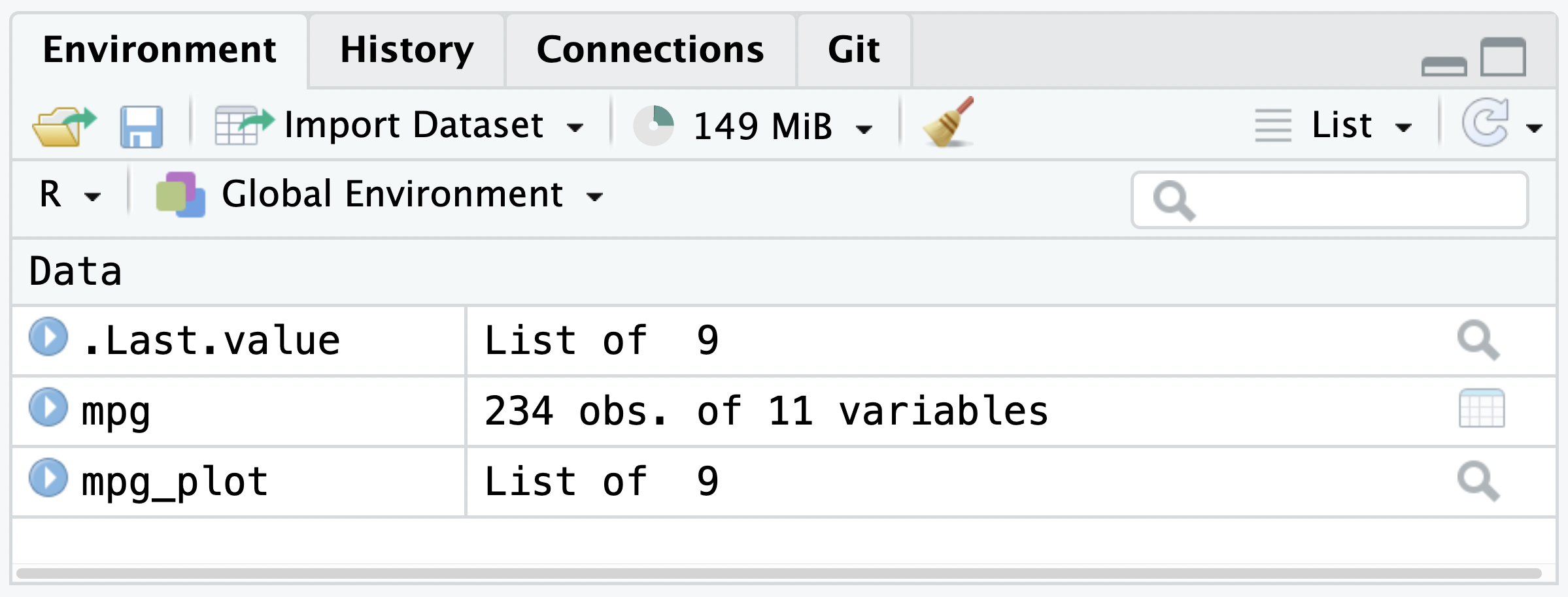
We can temporarily save this data frame object in R to our Environments pane by assigning it with the <- operator. Objects in the Environment pane are available for the duration of the current session, but are removed upon restarting R or RStudio.

As a beginning R user, it’s OK to consider your environment (i.e. the objects listed in the environment pane) “real”. However, in the long run, you’ll be much better off if you consider your R scripts as “real”. With your R scripts (and your data files), you can recreate the environment. It’s much harder to recreate your R scripts from your environment!

# this will temporarily assign the mpg dataset 
# to the mpg object in our current session
mpg <- ggplot2::mpg

Display the data

You can then display the first few rows of the mpg dataframe like so:

head(mpg)

#> # A tibble: 6 × 11
#>   manufacturer model displ  year   cyl trans      drv     cty   hwy fl    class  
#>   <chr>        <chr> <dbl> <int> <int> <chr>      <chr> <int> <int> <chr> <chr>  
#> 1 audi         a4      1.8  1999     4 auto(l5)   f        18    29 p     compact
#> 2 audi         a4      1.8  1999     4 manual(m5) f        21    29 p     compact
#> 3 audi         a4      2    2008     4 manual(m6) f        20    31 p     compact
#> 4 audi         a4      2    2008     4 auto(av)   f        21    30 p     compact
#> 5 audi         a4      2.8  1999     6 auto(l5)   f        16    26 p     compact
#> 6 audi         a4      2.8  1999     6 manual(m5) f        18    26 p     compact

Among the variables in mpg are:

displ, a car’s engine size, in liters.
hwy, a car’s fuel efficiency on the highway, in miles per gallon (mpg). A car with a low fuel efficiency consumes more fuel than a car with a high fuel efficiency when they travel the same distance.

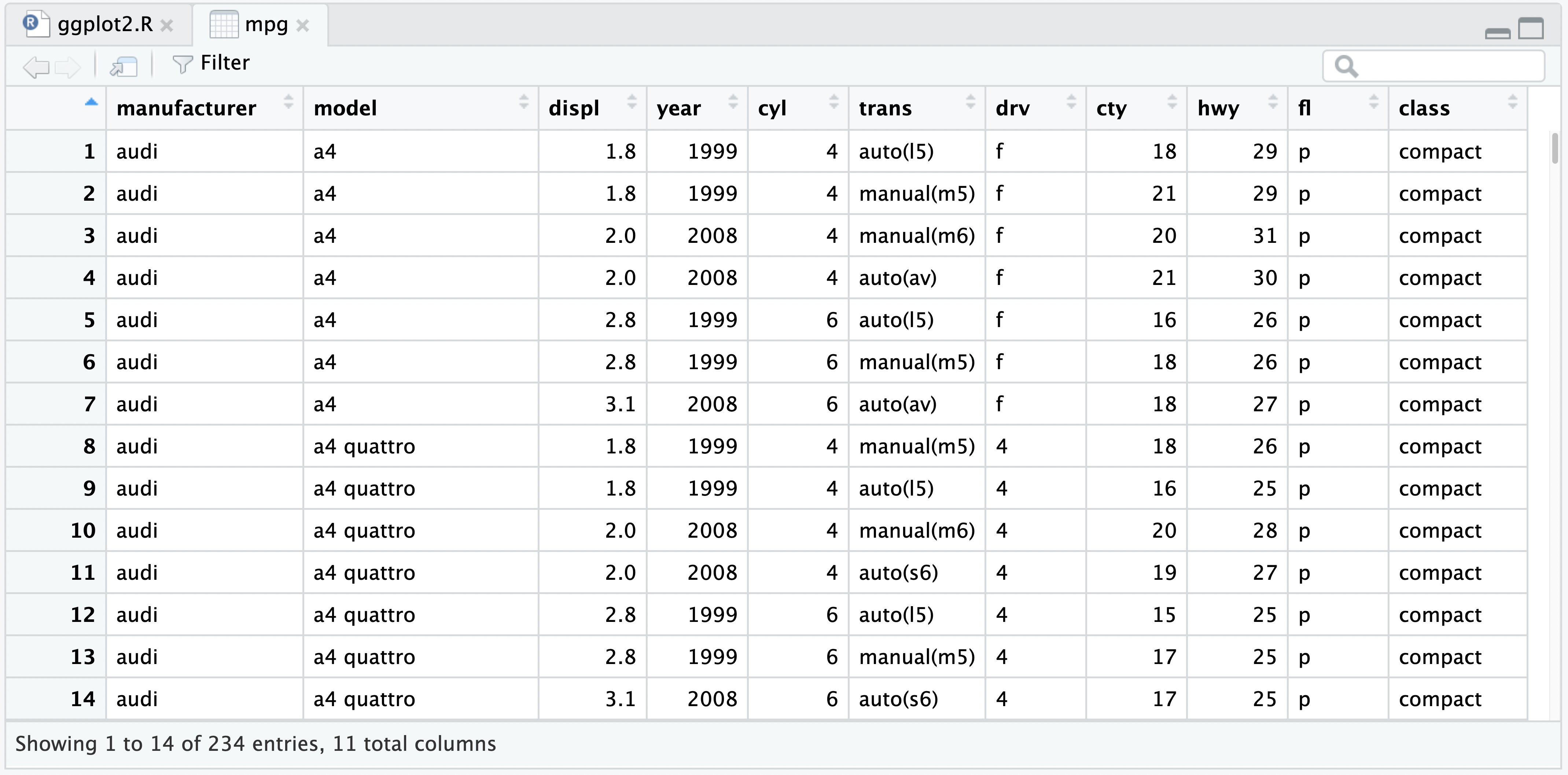
To get more of a spreadsheet “view” of the data, you can use the View() function:

View(mpg)

This will open up a new tab in the Source pane titled “mpg”. You can explore the data here interactively. To get back to your “ggplot2.R” file, select the ggplot2.R tab in the Source pane.

A screenshot of the output of `View(mpg)` which creates a spreadsheet-like view of the mpg dataset.

Create a graph

Next, in your ggplot2.R file in the source pane, you can type the following code:

mpg_plot <- ggplot(data = mpg, mapping = aes(x = displ, y = hwy)) +
  geom_point(mapping = aes(colour = class)) +
  geom_smooth(method = "lm", formula = "y ~ x")

Again, you will want to execute that by either the Run command or shortcut (Ctrl + Enter or Cmd + Enter on Mac). Note that we are using the <- operator to assign this plot to the mpg_plot object. The mpg_plot object will be visible in the top right Environment Pane.

A screenshot of the Environments pane, showing the mpg and mpg_plot objects

Print the graph

To print the graph in the Output Pane, we can add and then execute one more line of code:

mpg_plot

That will then display the plot into the Output Pane > Plots tab.

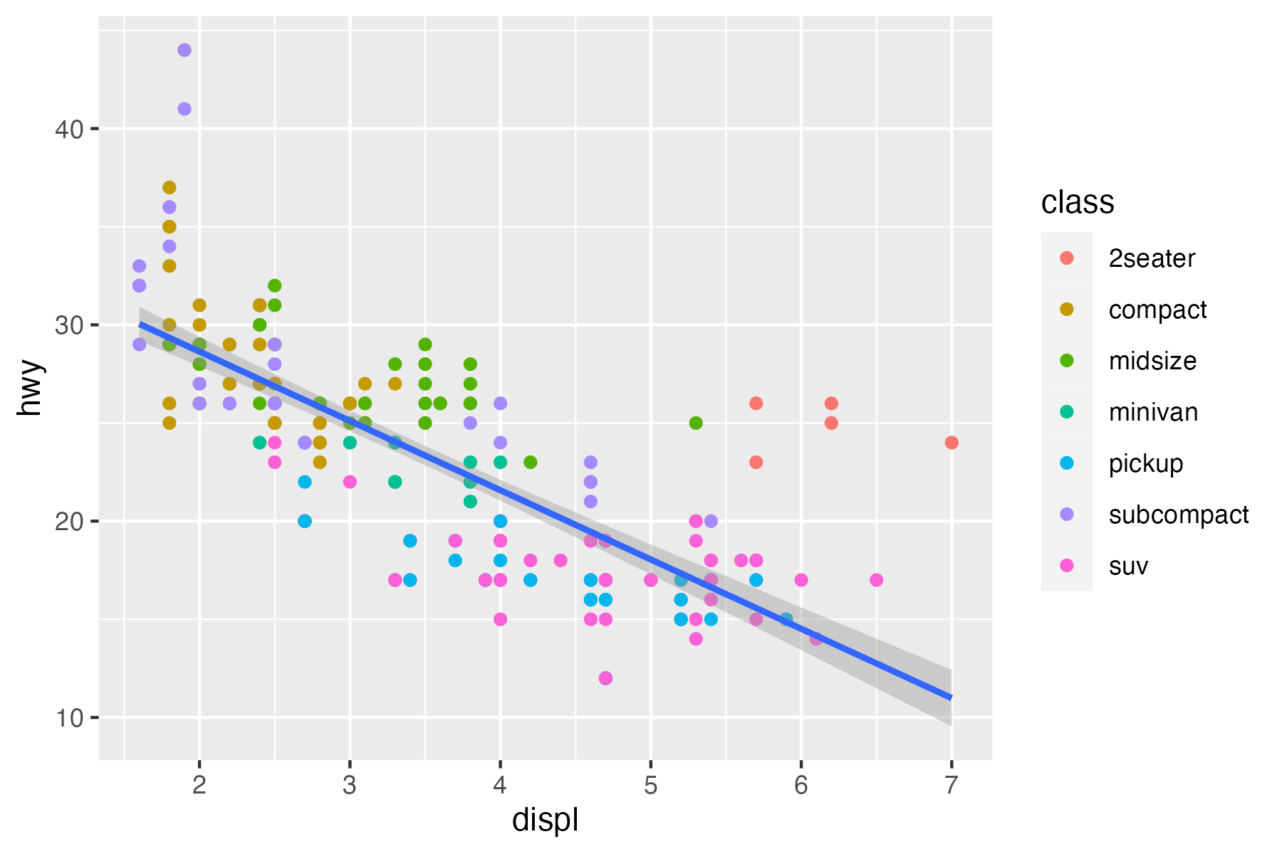
A ggplot of fuel displacement on the x-axis and highway miles per gallon on the y-axis. There is a negative, roughly linear relationship between mpg and displacement, as fuel displacement increases, the highway mpg decreases. The points are colored by class of vehicle, where pickups and SUVs have larger engines and worse fuel-efficiency than subcompact, compact, or midsize vehicles.

The plot shows a negative relationship between engine size (displ) and fuel efficiency (hwy). In other words, cars with smaller engine sizes have higher fuel efficiency and, in general, as engine size increases, fuel efficiency decreases. Does this confirm or refute your hypothesis about fuel efficiency and engine size?

Save the graph

Lastly, we may want to save this image as proof of our hardwork! We can use ggplot2 to save the image to disk with the below code or use the Export button in the Plot Pane.

ggsave("my-first-plot.png", plot = mpg_plot, height = 4, width = 6)

Now that the file has been saved to disk, we can find it by switching from the Plot tab to the Files tab, both of which are located by default in the Output Pane.

If you haven’t already, you should also save your ggplot2.R file at this point. From the Files Tab you can find your saved ggplot2 graph as “my-first-plot.png”, and if you have saved your ggplot2.R script - it will also be in this same folder.

Remember - with your R scripts and data files you can recreate this temporary session environment! To prove our point, after you have saved your ggplot2.R file, restart your session with the RStudio menu: Session > Restart R. Even in this fresh environment, you can recreate your plot by re-executing the source code with the same data!

Closing

While this exercise may have seemed simple, we have learned quite a few things about RStudio:

There are 4 core panes for managing data analysis tasks

The Source Pane is used to write longer scripts that can executed line-by-line or be saved to disk
The Console Pane is used to execute short interactive code
The Environment Pane is used to temporarily store session objects
The Output Pane contains the Plot tab which display graphs, and the Files tab which lets you explore source code and output files.

To go deeper on learning about ggplot2 and the rest of the tidyverse please see the R for Data Science textbook. R for Data Science is available in print or as a freely available website

To learn more about the RStudio, please continue exploring this User Guide!