Data Viewer

RStudio includes a Data Viewer that allows you to look inside data frames and other rectangular data structures. The viewer also allows includes some simple exploratory data analysis (EDA) features that can help you understand the data as you manipulate it with R or Python.

Starting the viewer

You can invoke the viewer in a console by calling the View function on the data frame you want to look at.

For example, to view the mpg dataset from ggplot2, execute these commands in the R console:

library(ggplot2)
mpg_df <- ggplot2::mpg[c("manufacturer", "model", "displ", "cty", "hwy")]
View(mpg_df)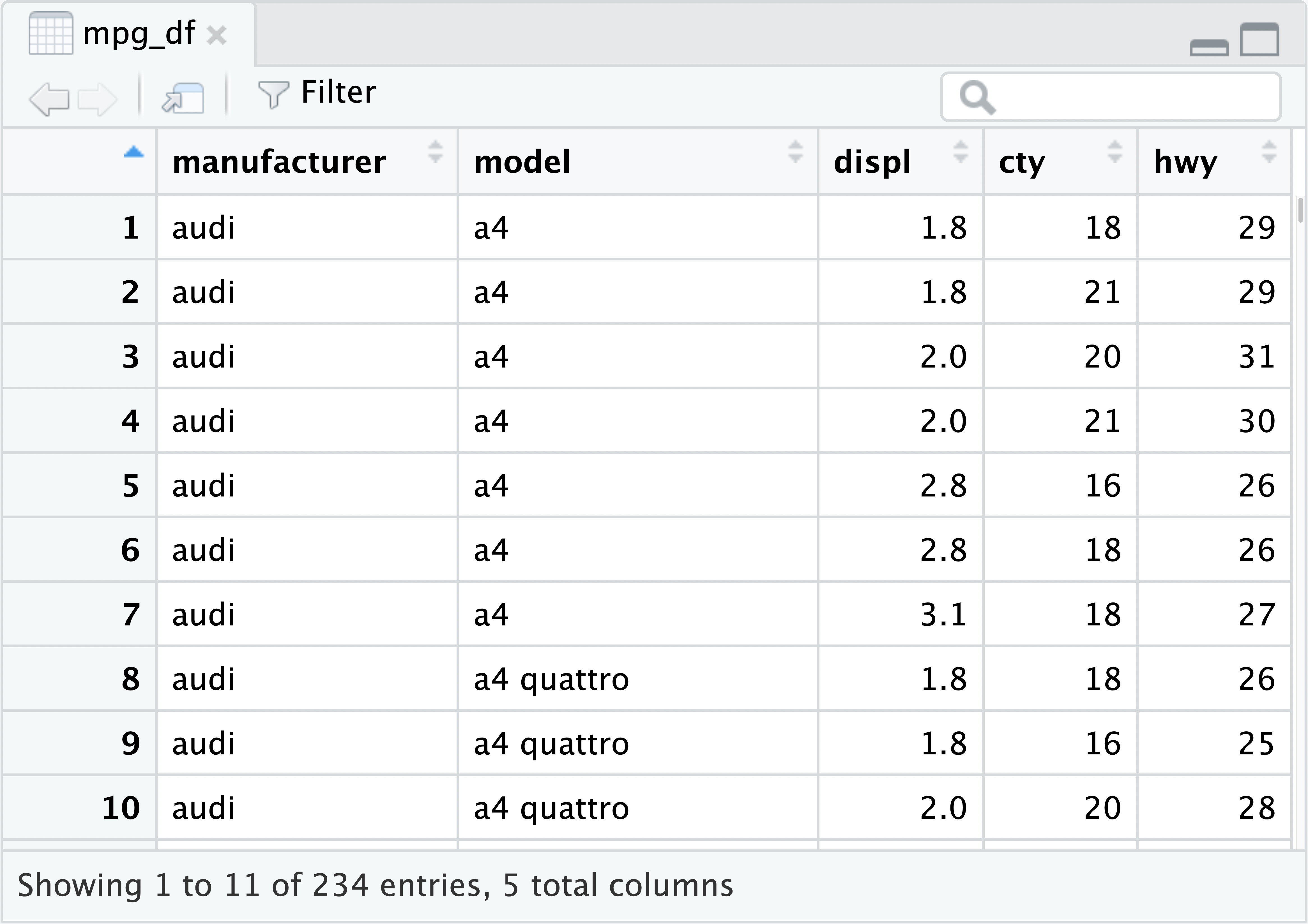

You can also start the viewer by clicking on the table data icon on the right, in the environment pane:

Sorting

You can sort by any column by clicking on the column label. Click on a column that is already sorted to reverse the sort direction.

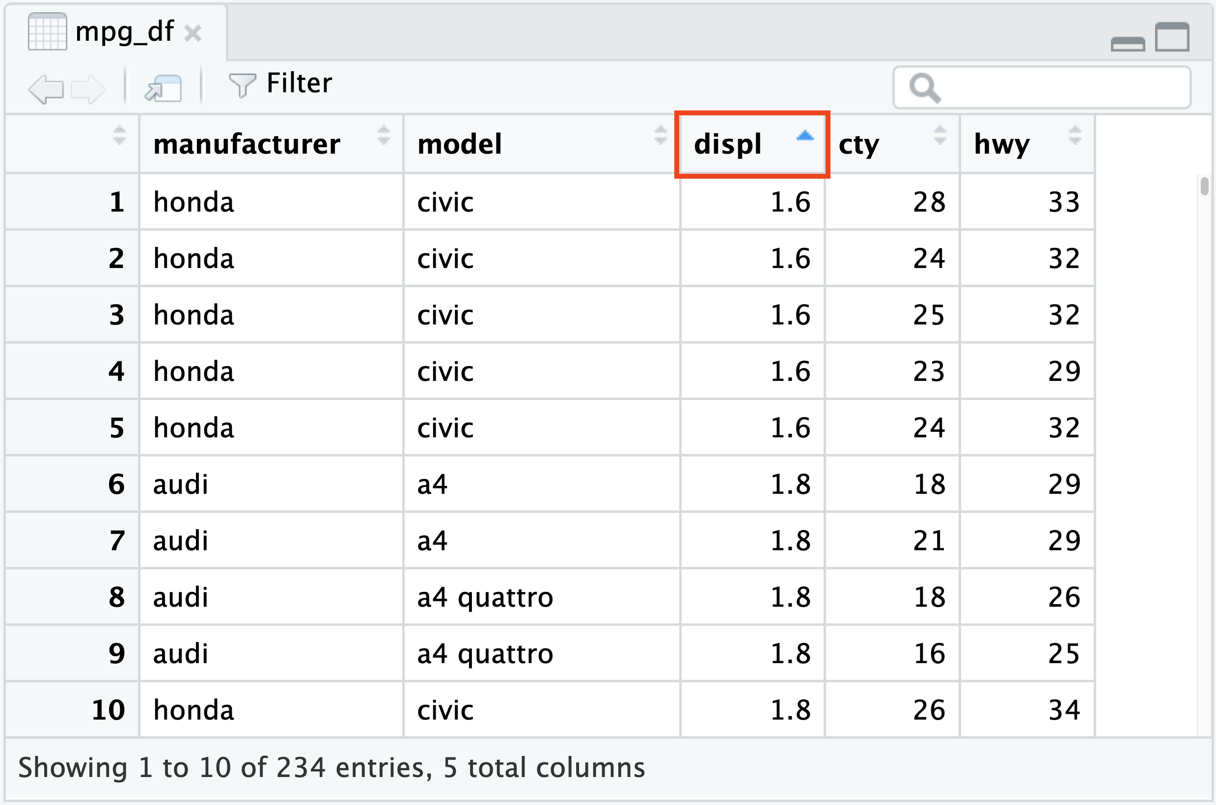
To remove sorting and show the data in the original order, click the empty column label cell in the upper left.

Scrolling

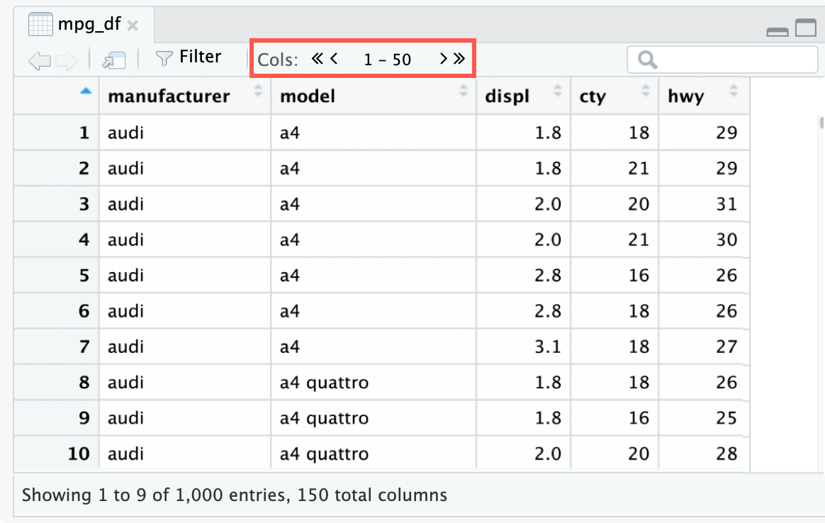
If you have more than 50 columns in your dataset, the data viewer only displays up to 50 columns. To view additional columns, click the single Cols > arrow to scroll right (columns display in groups of 50). If you want to jump to the end of your dataset, click the double Cols >> arrows.

Filtering

To apply filters, click the Filter icon in the toolbar. Any field that can be filtered will have a white box labeled All. Click this box to change which field values you want to see. For instance, to filter out cars with a highway fuel efficiency between 10 and 25 miles/gallon:

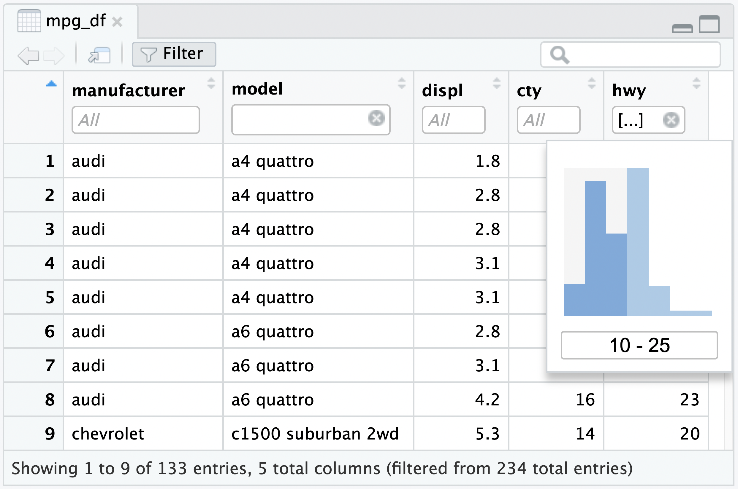
The Data Viewer includes a histogram filter or the raw values themselves can be modified. The text on the bottom of the pane indicates how many records the dataset contained before and after filtering; in this case we’ve filtered 234 records down to 133.

Not all kinds of fields can be filtered. At the moment, the following types are supported:

• Numeric

• Character

• Factor (treated as character if > 256 levels)

• Boolean (logical)

Filters are additive (i.e. joined with AND); that is, if you apply two column filters, you will see only records that match both of them.

Clear individual filters by clicking the (x) next to the filter; to clear all the filters at once, click the Filter icon in the toolbar.

Searching

You can search for text across all the columns of your frame by typing in the global filter box:

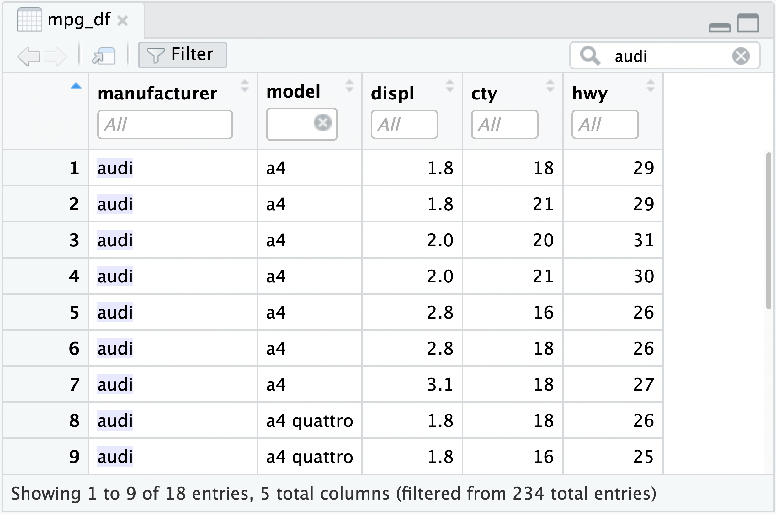
The search feature matches the literal text you type in with the displayed values, so in addition to searching for text in character fields, you can search for e.g. TRUE or 4.6 and see results in logical and numeric field types.

Searching and filtering are additive; when both are applied, you will see only records that match your filters and contain your search text.

Auto-refreshing

In most cases the viewer will automatically refresh itself if it detects that the underlying data has changed. Auto-refreshing works even when the Data Viewer is popped out into its own window.

As an example, execute this code:

data(Orange)
View(Orange)
Orange[1, "age"] <- 120

The age of the first tree change from 118 to 120 in the viewer.

This auto-refreshing feature has some prerequisites, so if it doesn’t seem to be working:

You must call View() on a variable directly. If, for instance, you call View(as.data.frame(foo)) or View(rbind(foo, bar)), you’re invoking View() on a new object created by evaluating your expression, and while that object contains data, it’s just a copy and won’t update when foo and bar do.

The variable must be in an environment in the search path ideally in the global environment.

Labels

The viewer supports column labels, such as those attached by the Hmisc package, by SPSS import from haven, or manually set via attr().

As an example, execute the below code:

attr(mpg_df$displ, "label") <- "engine displacement, in litres"
attr(mpg_df$cty, "label") <- "city miles per gallon"
attr(mpg_df$hwy, "label") <- "highway miles per gallon"
View(mpg_df)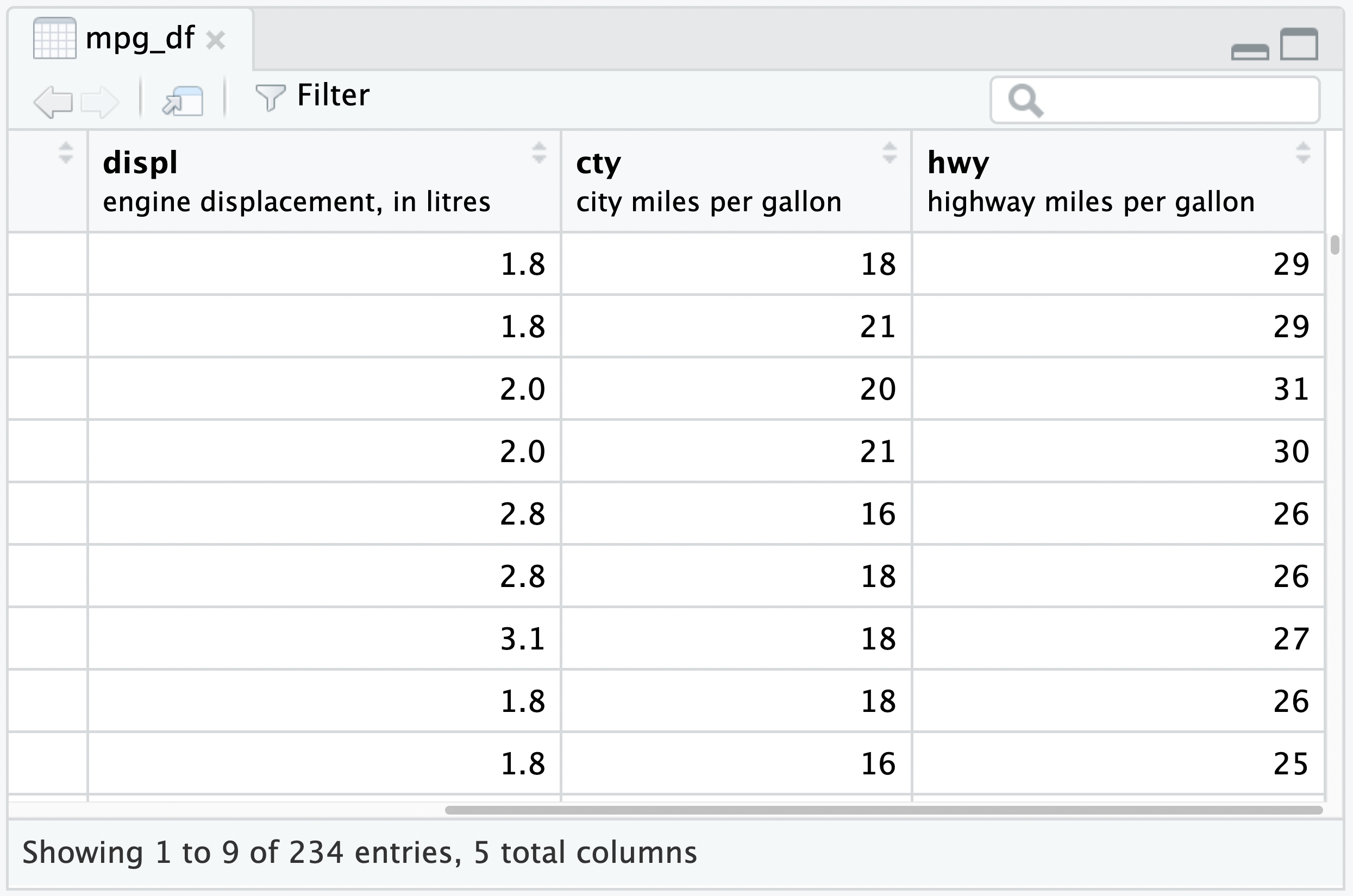

Both the label attribute on individual columns and the variable.labels attribute on the outer frame are supported.

Restrictions and performance

The number of rows the viewer can display is effectively unbounded, and large numbers of rows won’t slow down the interface. It uses the DataTables JavaScript library to virtualize scrolling, so only a few hundred rows are actually loaded at a time.

While rows and columns are unbounded, large numbers of columns may cause the interface to slow significantly.

Finally, while we’ve made every effort to keep things speedy, very large amounts of data may cause sluggishness, especially when a sort or filter is applied, as this requires R to fully scan the frame. If you’re working with large frames, try applying filters to reduce it to the subset you’re interested in to improve performance.

Lists and other objects

The Data Viewer can also operate on list() or JSON objects. This is very helpful for understanding the structure of deeply nested JSON.

Execute the following example:

my_list <- list(
  letters = list(a = 1, b = 2, c = 3),
  pets = list(c("dog", "cat", "lizard"))
)

View(my_list)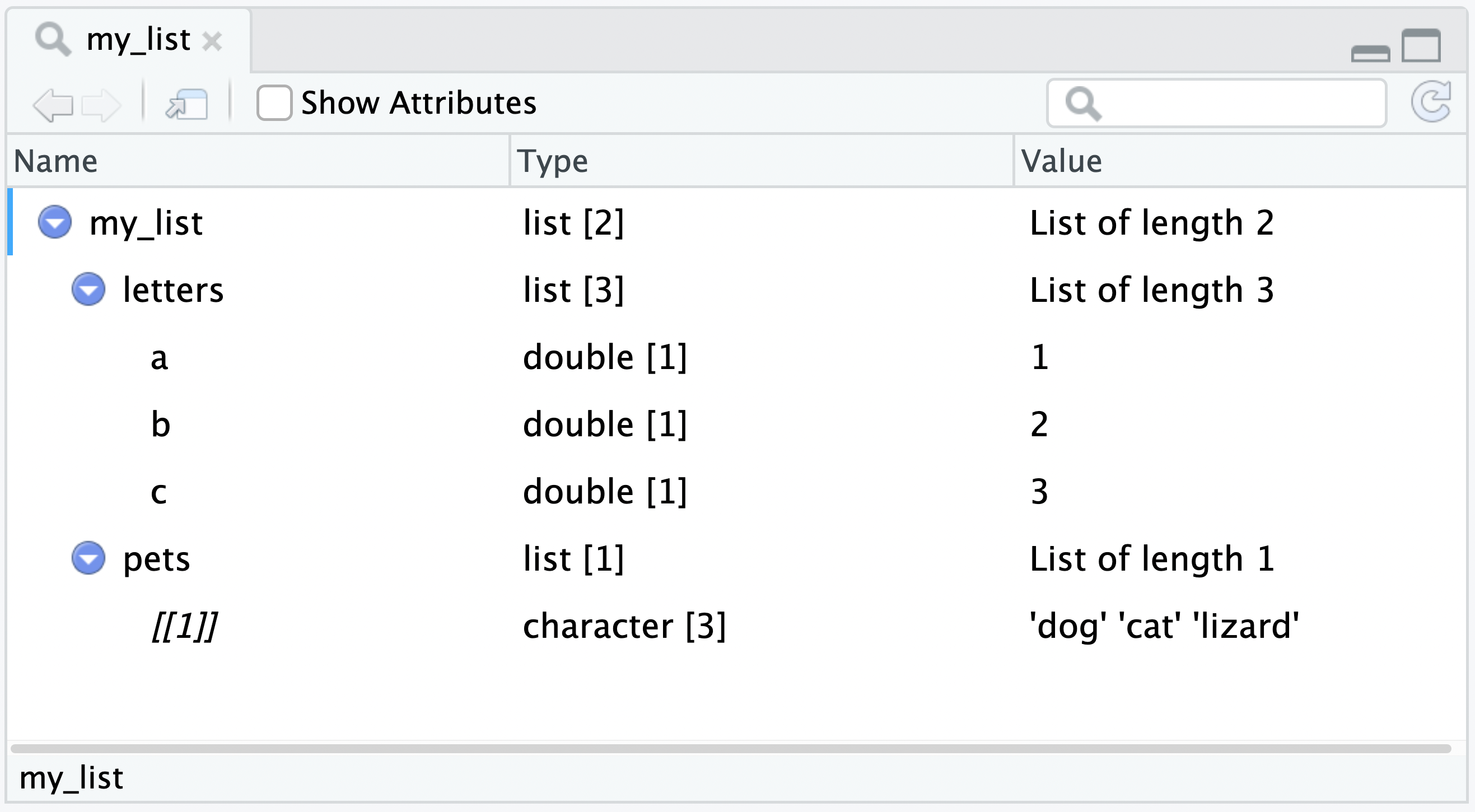

The Data Viewer also provides the ability to output the R code to extract a nested object.

Click on a specific line, and the Data Viewer will display the R code to extract that element, or click on the Send to Console icon to send the R code to the R console.

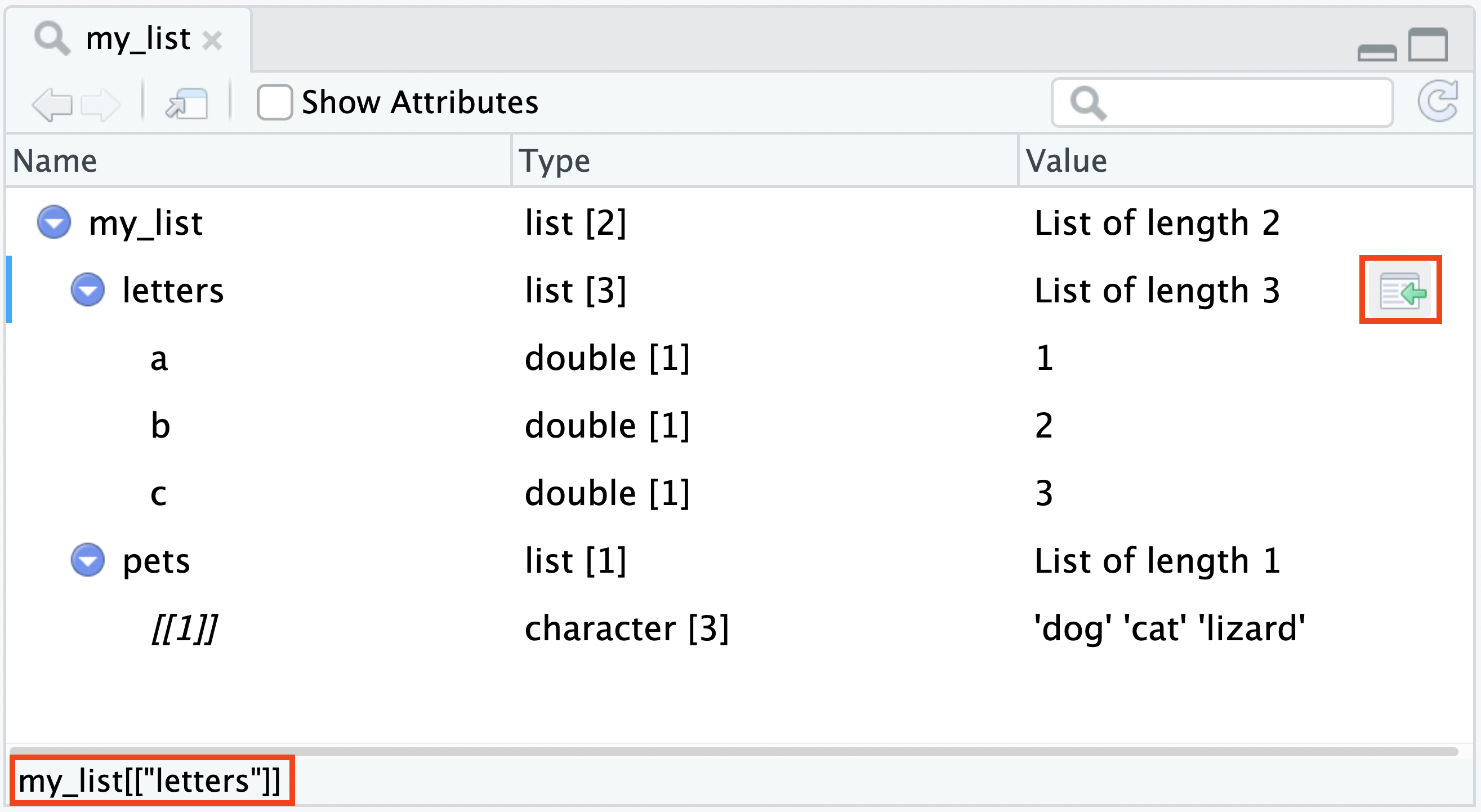The data can also be filtered with the search bar, providing a way to navigate larger or more deeply nested objects that will not easily fit on the page.