Jobs in action
As mentioned in RStudio Jobs, RStudio has the ability to send long running R scripts to local and remote background jobs. This functionality can dramatically improve the productivity of data scientists and analysts using R since they can continue working in RStudio while jobs are running in the background.
A few examples of integrating RStudio Jobs with specific development workflows in shiny, plumber, machine learning, or any long-running process are documented below.
Shiny app
Running a Shiny for R application as a local background job allows the current R session to remain free to work on other things. This can be especially helpful for making changes to the Shiny code and seeing the changes in real time.
A minimal example of running the Shiny app as a Job is documented below.
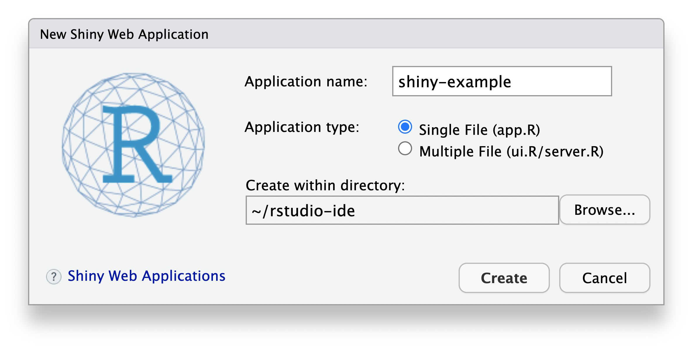
Use the RStudio global menu:
- File > New File > Shiny Web App...
- Set the Application Name: as “shiny-example”
- Set the Application Type: as a Single File (app.R)
This workflow will create a new folder titled “shiny-example” and populate it with a Shiny app.R file. In the same folder (“shiny-example”) as the newly created app.R, create a second .R file titled shiny-local.R with the following example code:
options(shiny.autoreload=TRUE)
shiny::runApp()
The shiny.autoreload=TRUE option provides the real-time updating of the Shiny app code without requiring an explicit reload of the Shiny app, and the shiny::runApp() code enables running all the Shiny components within the “shiny-example” folder. Sourcing as a shiny-local.R from within the same directory as a Shiny app.R will allow them to interact, using shiny-local.R to modify the behavior of the Shiny hosting.
The purpose of this two-file system is that you have a ready to deploy Shiny app (app.R) and a way to interactively test it locally (shiny-local.R) prior to deploying to production.
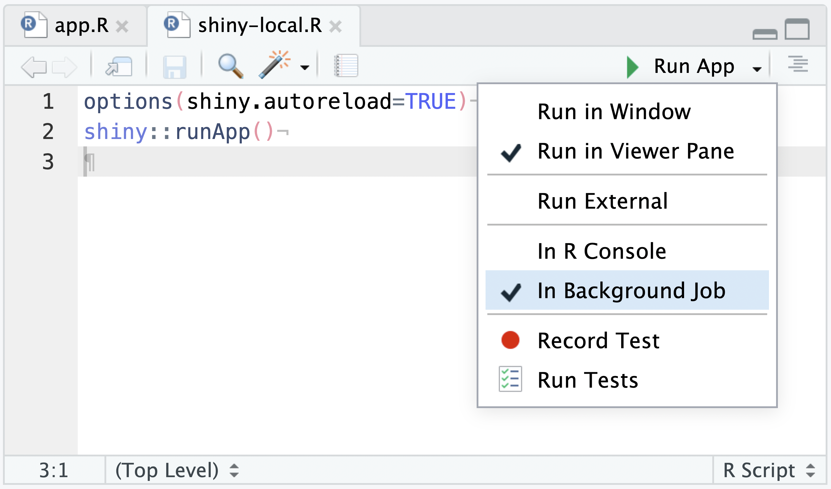
The shiny-local.R source file will have a Run App drop-down menu. From the Run App drop-down, select In Background Job and then press the Run App button:
With In Background Job set, the Run App button will execute the Shiny app in a Background Job, and automatically present it in the Viewer Pane:
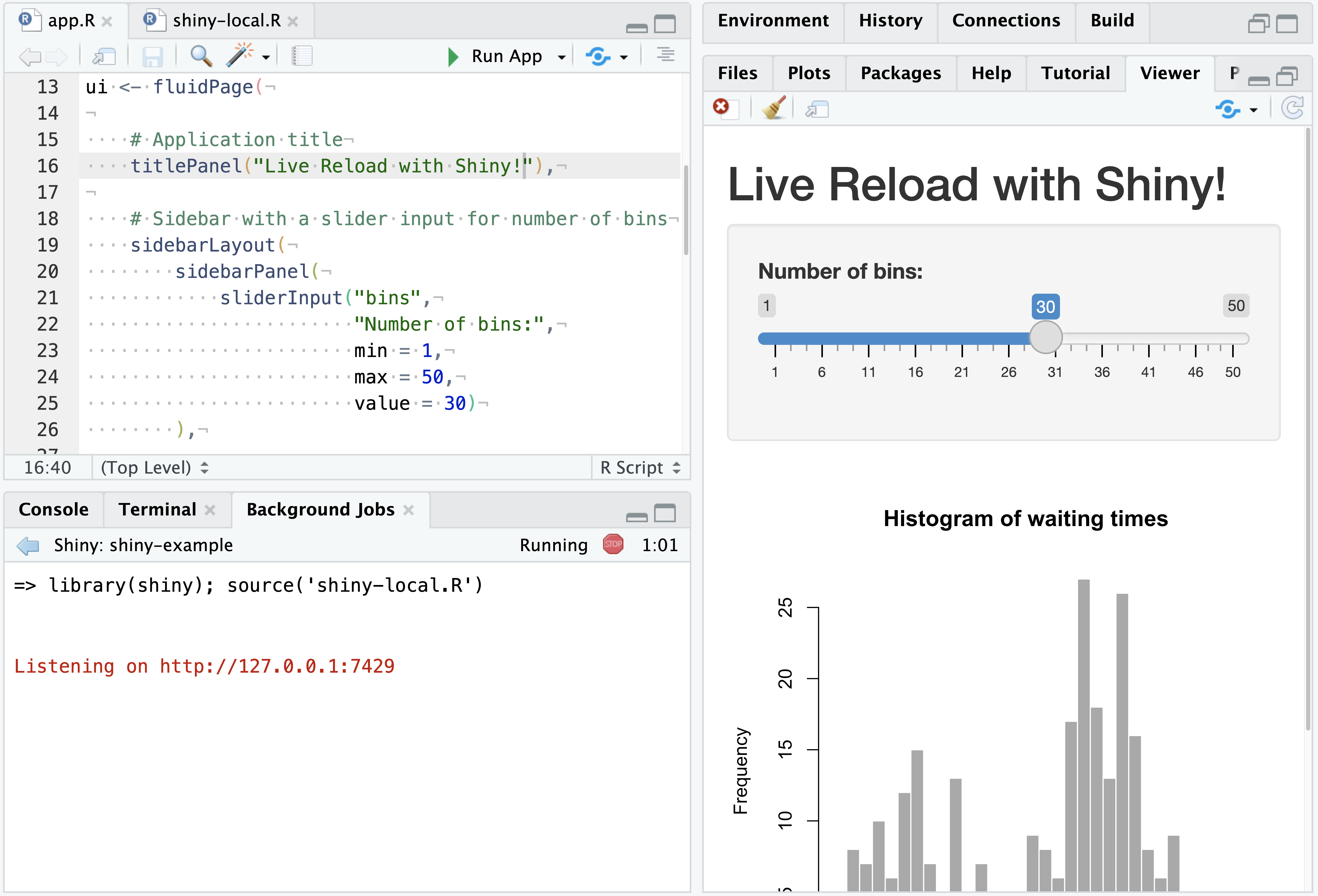
Working with Shiny apps in this way allows for interactive editing and updating of the displayed Shiny app in real time - both for Shiny user interface and server components.
Reload app
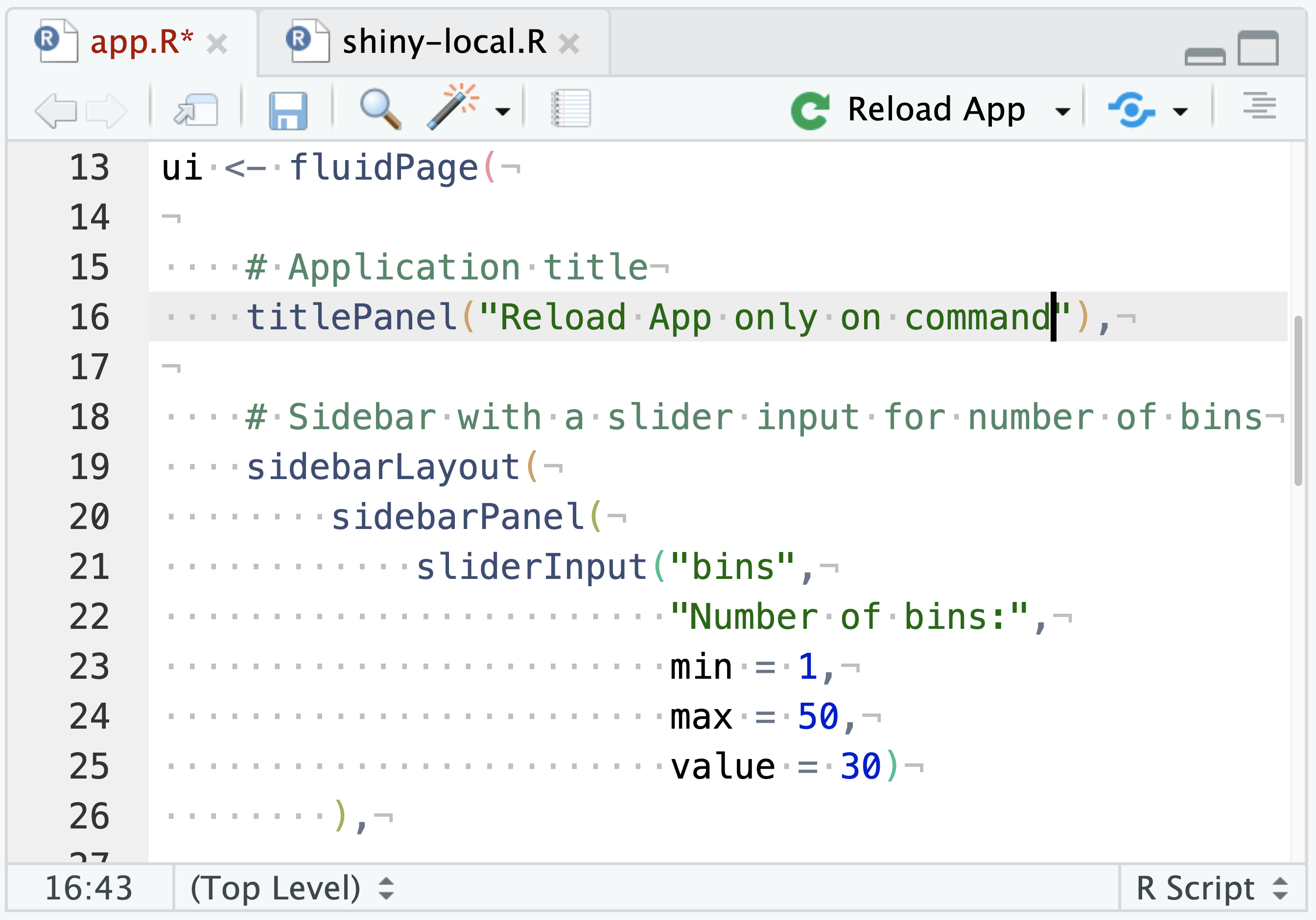
Alternatively, in the Shiny app.R file, there will also be a Run App drop-down. From Run App, select In Background Job and then press the Run App button. This will not have auto-reloading but might be preferable for Shiny apps with a long startup time.
In this scenario, after making changes to the app.R file, the Run App button will be replaced with a Reload App button. The Shiny app will still be executed in a Background Job, but the user must explicitly reload the app after making changes and press the Reload App button, rather than the auto-reload behavior in the previous example.
Plumber API
Similar to Shiny applications, plumber APIs can be run as a local background job. This allows the current R session to remain open for things like testing or interacting with the API via curl or R packages for querying APIs such as httr. plumber v1.1.0 or later is required for the below documentation.
If necessary, install the latest version of plumber and rapidoc from CRAN:
install.packages(c("plumber", "rapidoc))A minimal example of running a plumber API as a Job is documented below:
Use the RStudio global menu: File > New File > Plumber API... and save it as plumber-example.
In the same directory as plumber.R, create a second .R file titled plumber-local.R with the following example code:
library(plumber)
library(rapidoc)
pr("plumber.R") %>%
pr_set_docs("rapidoc") %>%
pr_set_docs_callback(rstudioapi::viewer) %>%
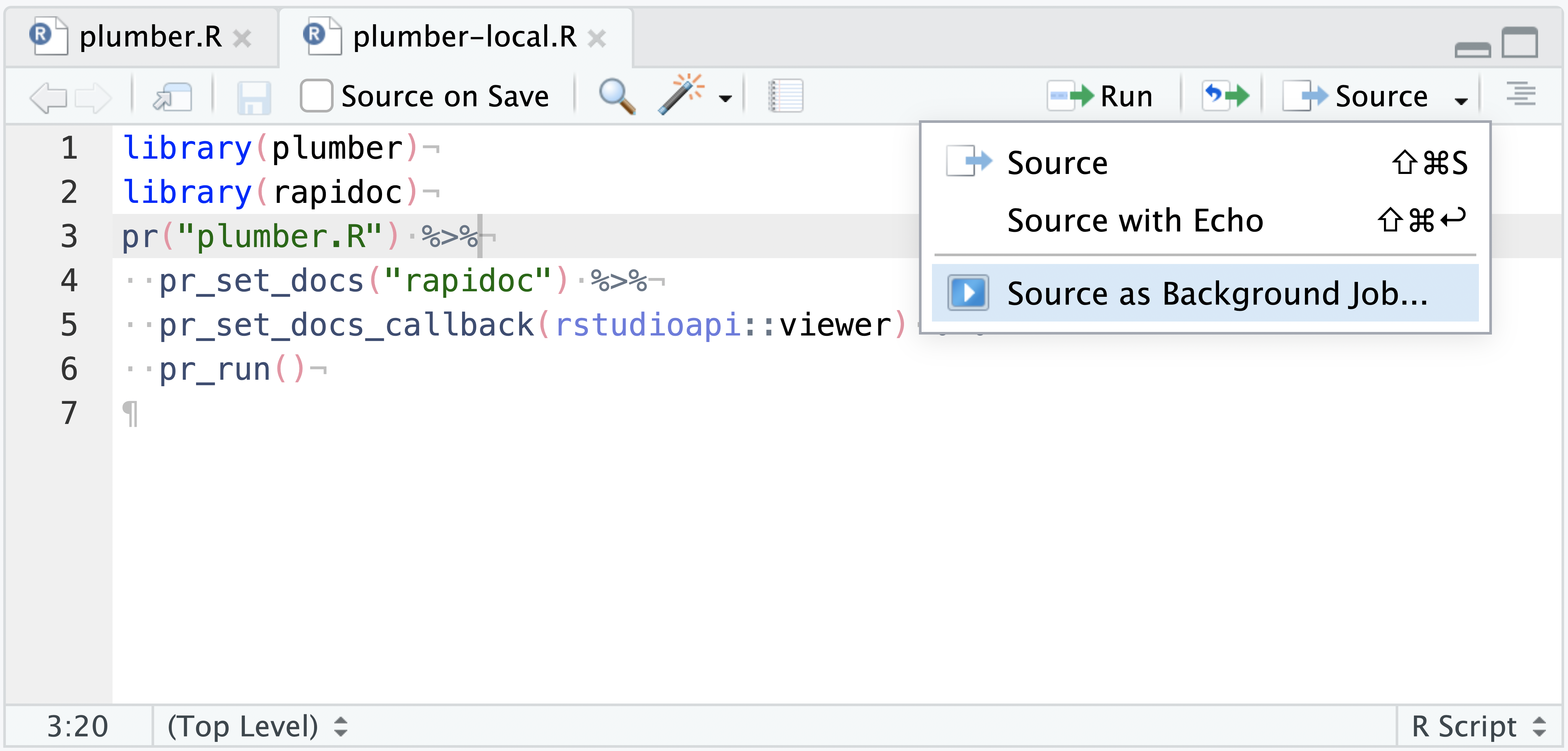
pr_run()This code will take an example plumber API, set rapidoc as the interactive documentation, and send the docs to the RStudio Viewer pane. The purpose of this two-file system is that you have a ready to deploy plumber API (plumber.R) and a way to interactively test it locally (plumber-local.R) prior to deploying to production.
Execute it as a Job from the Source pane via the Source > Source as a Background Job drop-down option.
In the upper-right corner of the RStudio Viewer pane, press the Refresh Viewer ![]() . This will display the plumber API’s rapidoc interface in the Viewer pane, allowing for interactive testing with the active plumber API in real time.
. This will display the plumber API’s rapidoc interface in the Viewer pane, allowing for interactive testing with the active plumber API in real time.
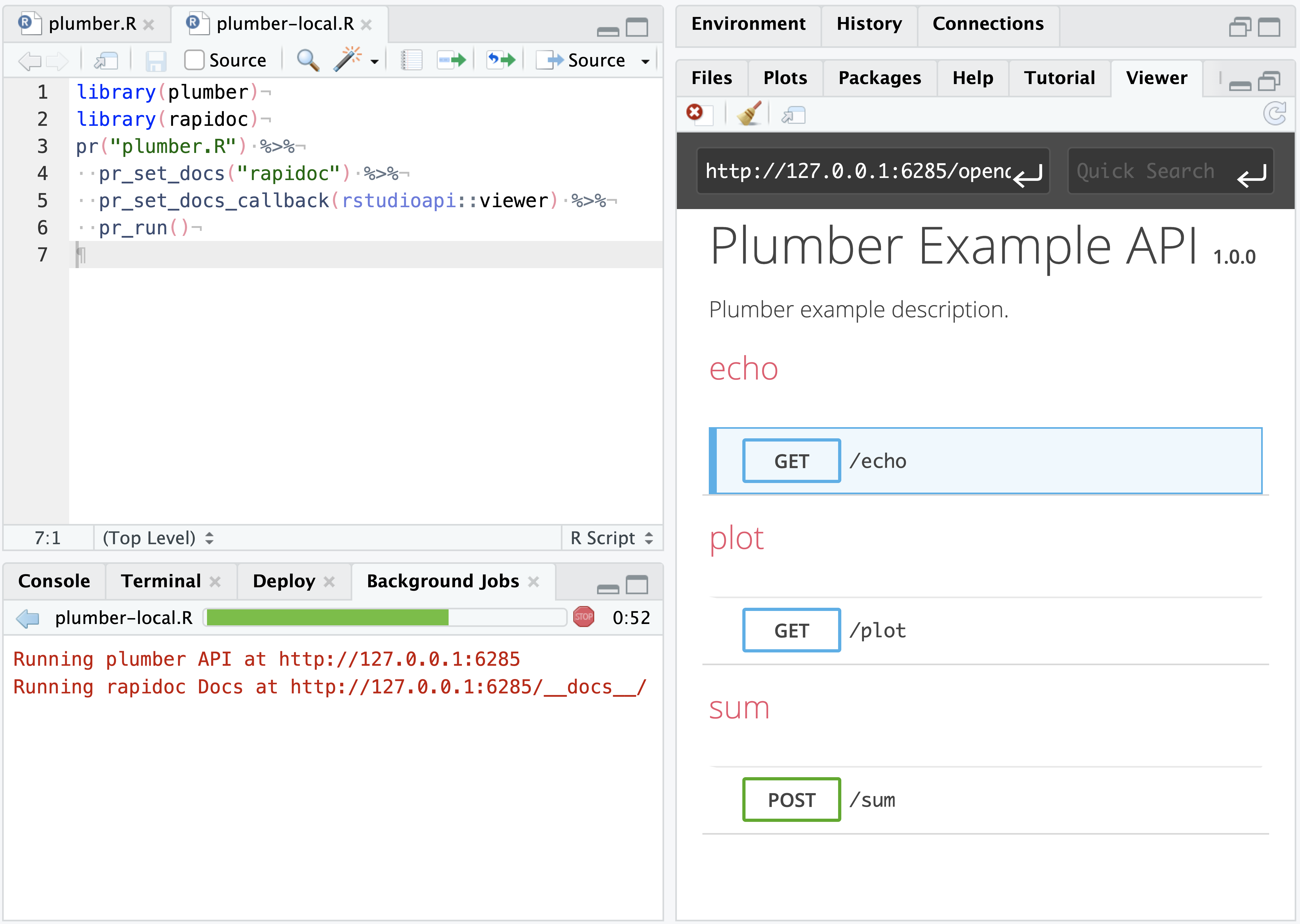
To interact with the API programatically in RStudio, use a R package such as httr or a command line tool such as curl. The example API has a few endpoints (/sum, /echo, /plot) and you can query them with GET() or POST() commands.
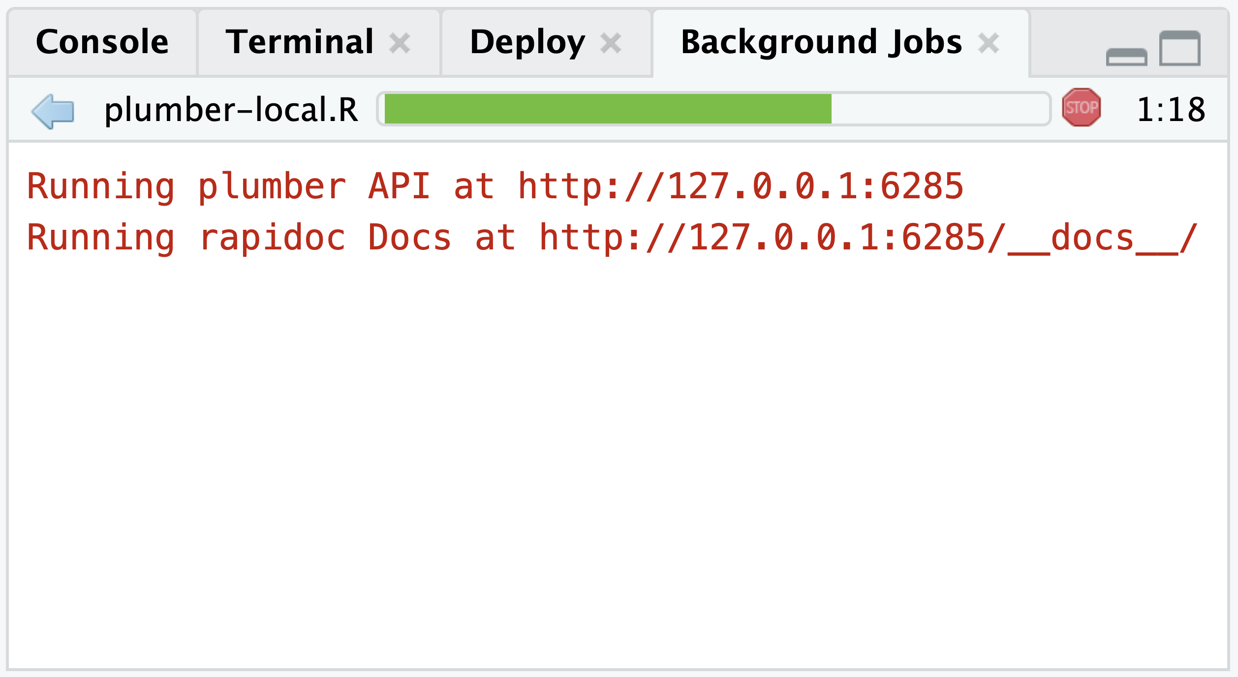
# if needed install.packages("httr")From the Background Jobs tab within the Console pane, the running API will return the URL to the API and it’s rapidoc Docs:
# This is an example URL and
# it will vary between sessions
Running plumber API at http://127.0.0.1:6285
Running rapidoc Docs at http://127.0.0.1:6285/docs/
We can add specific endpoints to that URL (http://127.0.0.1:6285) such as /sum or /echo and then query them with the httr package.
post_sum <- httr::POST("http://127.0.0.1:6285/sum", query = list(a=1, b = 2))

httr::content(post_sum)
#> [1] 3
get_echo <- httr::GET("http://127.0.0.1:6285/echo", query = list(msg = "dog"))
httr::content(get_echo)
#> $msg
#> [1] "The message is: 'dog'"vetiver model as an API
The vetiver framework is for MLOps tasks in Python and R. The vetiver R package has functions for deploying vetiver models as plumber APIs. This allows for remote deployment, as well as local testing in a similar way to generic plumber APIs. The vetiver example below is taken from the vetiver ‘Get Started’ documentation.
If necessary, install the latest versions of these packages from CRAN:
install.packages(c("tidymodels", "vetiver", "pins", "plumber"))First, save the below code as vetiver-train.R and execute it to generate a vetiver model and write out that model to a plumber API.
library(tidymodels)
library(vetiver)
library(pins)

car_mod <-
    workflow(mpg ~ ., decision_tree(mode = "regression")) %>%
    fit(mtcars)
v <- vetiver_model(car_mod, "cars_mpg")
model_board <- board_folder("pins-r", versioned = TRUE)
model_board %>% vetiver_pin_write(v)

# write out a vetiver model to a plumber API
vetiver_write_plumber(model_board, "cars_mpg", file = "vetiver-plumber.R")
Create and save a second file as vetiver-local.R with the code below:
# vetiver-local.R
library(plumber)
library(vetiver)

pr("vetiver-plumber.R") %>%
  pr_set_docs_callback(rstudioapi::viewer) %>%
  pr_run()
The vetiver-local.R file can be run as a Background Job like any other plumber API, hosting the vetiver model as an API temporarily. The purpose of this two-file system is that you have a ready to deploy vetiver model as a plumber API (vetiver-plumber.R) and a way to interactively test it locally (vetiver-local.R) prior to deploying to production.
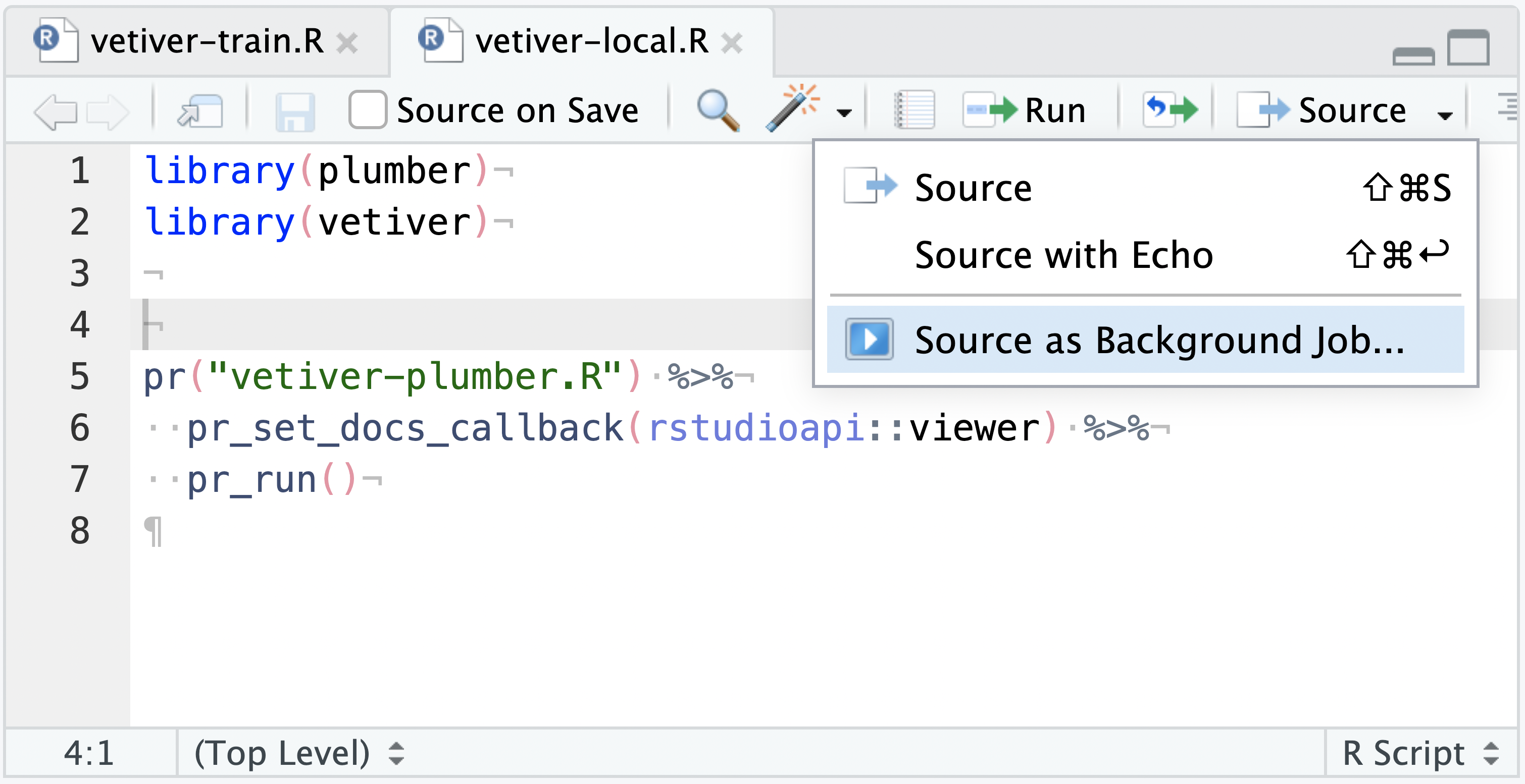
If you don’t want to write out the plumber API yet, you can also launch a vetiver API directly with vetiver. This requires selecting Run job with copy of global environment when pressing Source as Background Job, as the vetiver_model() exists in the global environment as v in the current example:
pr() %>%
  pr_set_docs_callback(rstudioapi::viewer) %>%
  # use the existing vetiver_model object 'v'
  vetiver_api(v) %>%
  pr_run()
From the Source drop-down menu, select Source as Background Job. This will launch the API as a Background Job.
In the upper-right corner of the RStudio Viewer pane, press the Refresh Viewer ![]() . This will display the API’s interface in the Viewer pane, allowing for interactive testing of the temporarily hosted vetiver model in real time.
. This will display the API’s interface in the Viewer pane, allowing for interactive testing of the temporarily hosted vetiver model in real time.
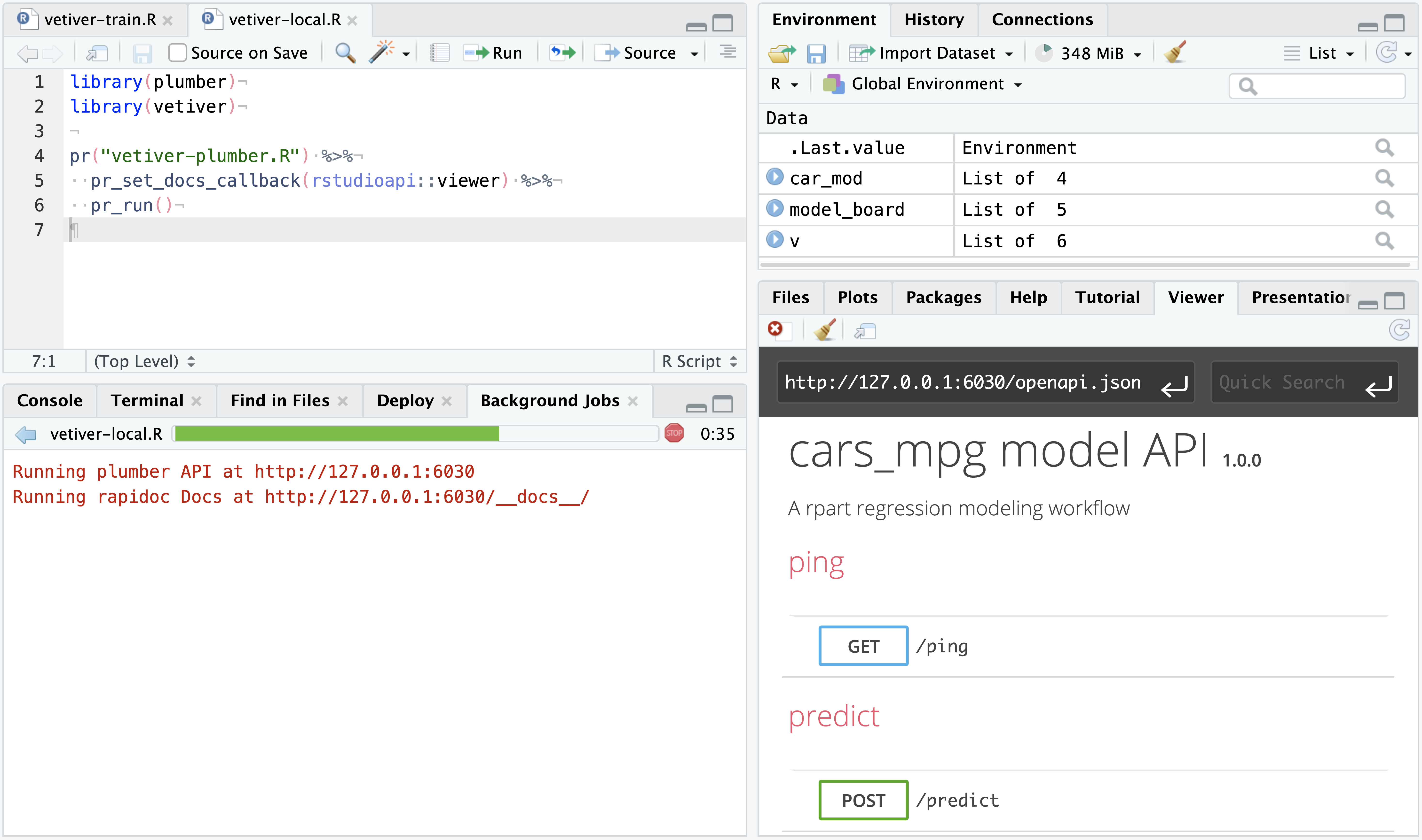
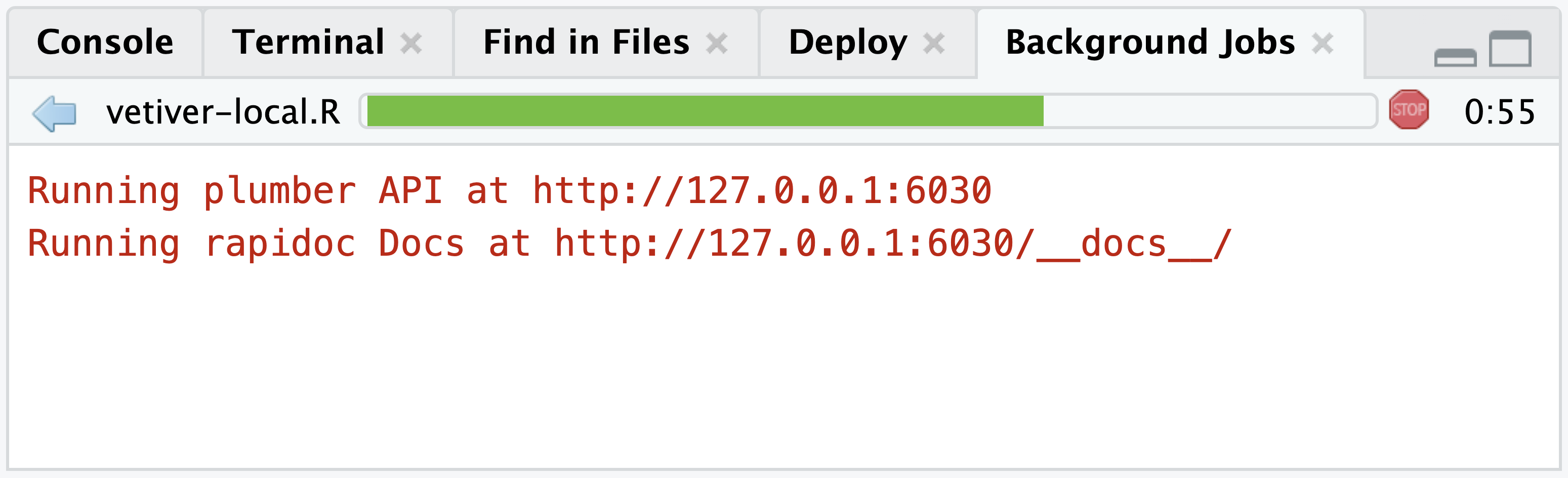
You can also programatically send new data and test new predictions with the vetiver model. In the Background Jobs tab within the Console pane, the active API will return the URL to the API and it’s rapidoc Docs.
# This is an example URL and
# it will vary between sessions
Running plumber API at http://127.0.0.1:6030
Running rapidoc Docs at http://127.0.0.1:6030/__docs__/
Add the /predict endpoint to the end of the URL and save it as a vetiver_endpoint().
endpoint <- vetiver_endpoint("http://127.0.0.1:6030/predict")You can then make predictions with new data for that model running in the separate Background Job process.
new_car <- tibble(cyl = 4,  disp = 200,
                  hp = 100, drat = 3,
                  wt = 3,   qsec = 17,
                  vs = 0,   am = 1,
                  gear = 4, carb = 2)
predict(endpoint, new_car)

#> # A tibble: 11 × 1
#>    .pred
#>    <chr>
#>  1 22.3
Extract, transform, load (ETL)
Background and Workbench Jobs are ideal for long running processes, like interactively loading data from an external database or API. Non-interactive, scheduled ETL scripts should be handled by Posit Connect.
Simulations
Long running tasks like simulation studies can be run as background or Workbench Jobs in order to keep the original R session open for other work.
For example - a Monte Carlo simulation for estimating pi could be saved as simulate-pi.R:
simulate-pi.R Code
# Use a monto carlo simulation to estimate pi
n <- 1e6
if (!dir.exists("output")) dir.create("output")
results_file <- tempfile("pi-", "output", ".rds")
results <- matrix(nrow = n, ncol = 2)
for (i in 1:n){
results[i,] <- runif(2)
# save out results every 25 iterations
if (i %% 25 == 0) {
print(paste0("Saving results (i = ", i, ")"))
save_results <- results[apply(results, 1, function(x) !all(is.na(x))),]
print(
paste0(
"Pi estimate: ",
mean((save_results[,1]^2 + save_results[,2]^2) <= 1) * 4)
)
saveRDS(save_results, results_file)
}
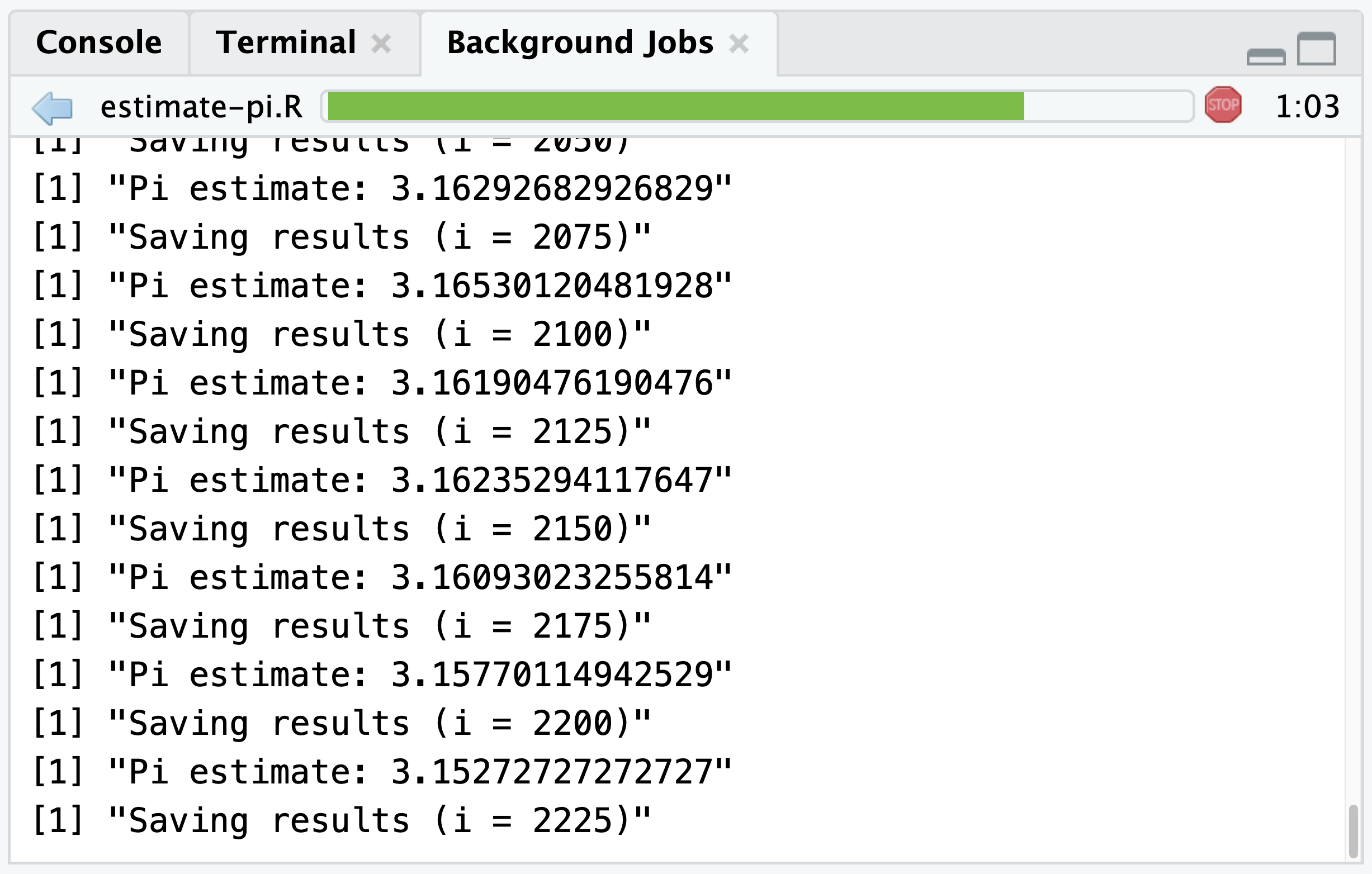
}This script includes:
print()calls for each 25 runs and the estimation of pi at that moment in timesaveRDS()to save out and overwrite the results after each 25 runs
Executing this script as a Job with the included print() calls will display the current estimated value of Pi and a running number of simulations in the Background Jobs pane:
Model training
Model training and tuning, which can often take a long time, is another great use case for background and Workbench Jobs. Local jobs are ideal for sequential model training while Workbench Jobs can be used to train multiple models in parallel on elastic scaling infrastructure.
The example script at https://tune.tidymodels.org/reference/example_ames_knn.html can be executed as a background or Workbench Job, enhanced with one modification.
Add control = control_grid(verbose = TRUE) to the tune_grid() step:
ames_grid_search <-
tune_grid(
ames_wflow,
resamples = rs_splits,
grid = ames_grid,
# this will print each step of the tuning process
control = control_grid(verbose = TRUE)
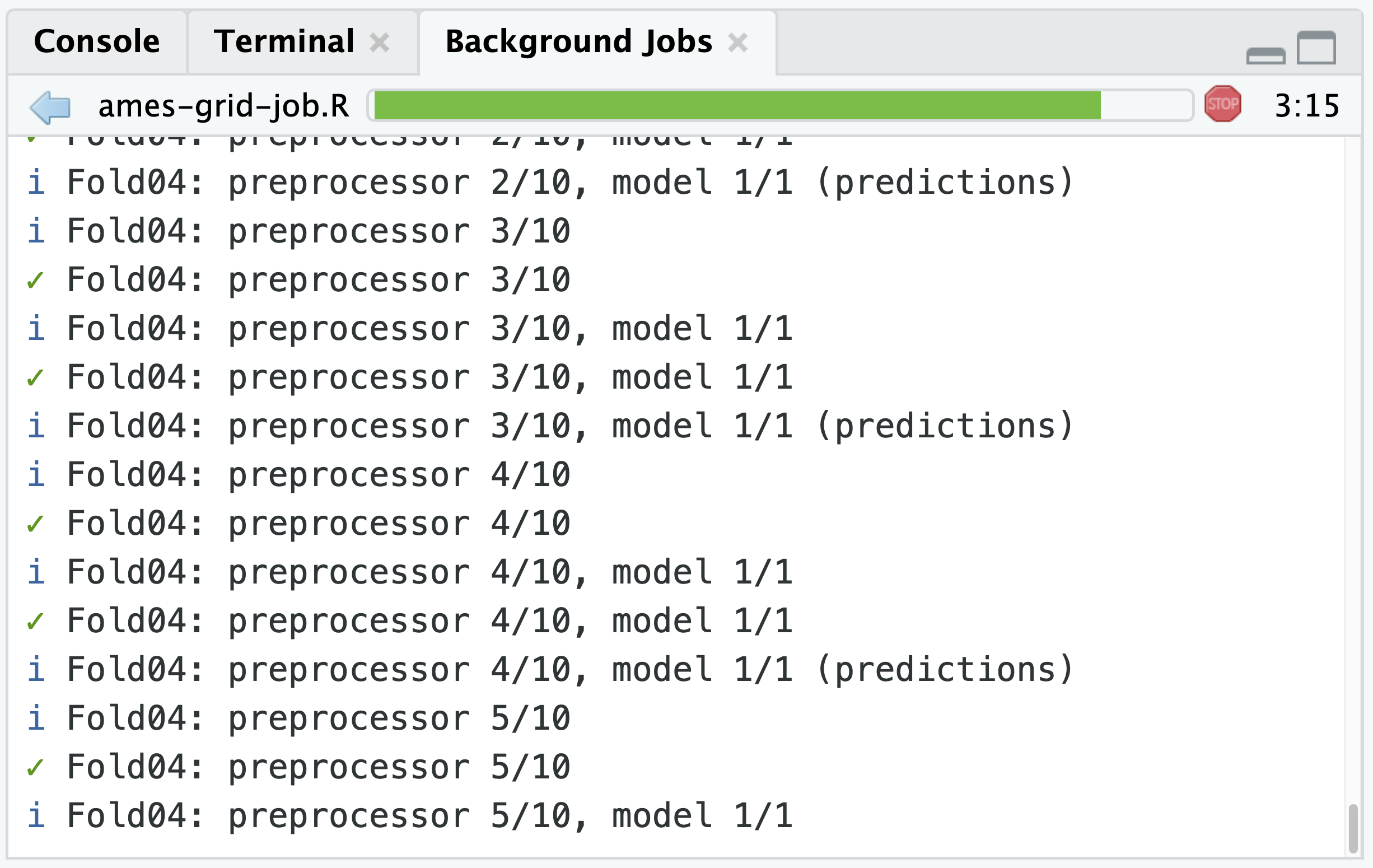
)Including the control_grid(verbose = TRUE) means the output from that grid tuning of a tidymodels workflow will print and update wherever it is being executed, including the Background Jobs tab. For this code it will print the current fold and split:
Programmatic Jobs
The above documentation has focused on using the RStudio user interface to kick off and interact with Jobs. The rstudioapi package provides tools for programmatically creating local and Workbench jobs.
Local Background Jobs
| Interact with the jobs pane. | |
|---|---|
jobAdd() |
Add a Job |
jobAddOutput() |
Add Background Job Output |
jobAddProgress() |
Add Background Job Progress |
jobRemove() |
Remove a Background Job |
jobRunScript() |
Run R Script As Background Job |
jobSetProgress() |
Set Background Job Progress |
jobSetState() |
Set Background Job State |
jobSetStatus() |
Set Background Job Status |
Workbench Jobs
| Interact with the Workbench Jobs pane. | |
|---|---|
launcherAvailable() |
Check if Workbench Launcher is Available |
launcherConfig() |
Define a Workbench Launcher Configuration |
launcherContainer() |
Define a Workbench Launcher Container |
launcherControlJob() |
Interact with (Control) a Workbench Job |
launcherGetInfo() |
Retrieve Workbench Launcher Information |
launcherGetJob() |
Retrieve Workbench Job Information |
launcherGetJobs() |
Retrieve Workbench Job Information |
launcherHostMount() |
Define a Workbench Launcher Host Mount |
launcherNfsMount() |
Define a Workbench Launcher NFS Mount |
launcherPlacementConstraint() |
Define a Workbench Launcher Placement Constraint |
launcherResourceLimit() |
Define a Workbench Launcher Resource Limit |
launcherSubmitJob() |
Submit a Workbench Job |
launcherSubmitR() |
Execute an R Script as a Workbench Job |